01 / Context & question
A glass fragment can guide an investigation, provided we know what kind of glass it is.
Each sample is described by its refractive index (RI) and its content of eight elements: sodium (Na), magnesium (Mg), aluminium (Al), silicon (Si), potassium (K), calcium (Ca), barium (Ba) and iron (Fe). The task is to predict its type among six.
The classification scheme has seven types, but no non-float vehicle-window sample (Type 4) exists in the data, so the problem has six classes.
With so few samples, which model classifies the six types best, and which ones remain hard to separate?
Before comparing models, I needed to understand the shape of these 214 rows.
02 / What the data shows before modeling
Barium strongly separates headlamps, while several window-glass types remain chemically close.
Headlamp fragments show clearly higher barium levels.
Containers and headlamps show little magnesium compared with several building-window classes.
Their chemistry overlaps more, foreshadowing the errors later visible in the confusion matrix.
Why this matters: EDA is not only preprocessing. It already explains why some classes are easier to recognize and others remain ambiguous.
03 / Exploratory data analysis (EDA)
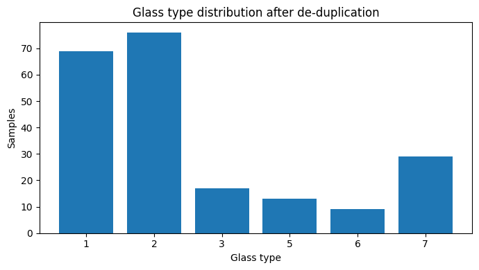
Exploration reveals a tiny, very imbalanced dataset with extreme values that may well be real.
Exploratory data analysis (EDA) means examining the data before any modelling: counts, duplicates, distributions, extreme values and visible differences between classes. Here it decides both how the models must be evaluated and what can be expected from them.
- missing values and duplicates;
- number of samples per type;
- distribution of each measurement and extreme values;
- correlations between measurements;
- chemical profiles that set some types apart.
214 rows, one exact duplicate removed.
Type 2, non-float windows.
Type 6, tableware.
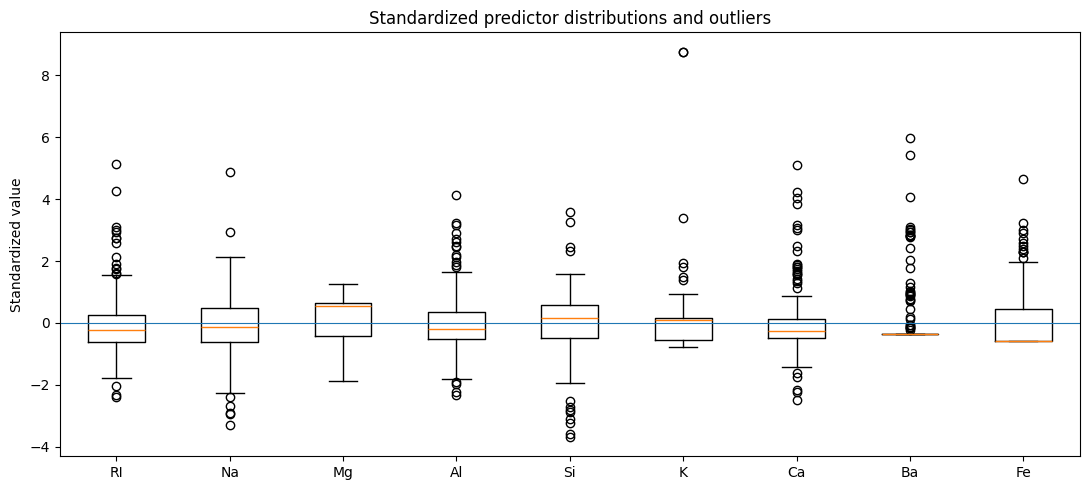
I kept the extreme values: in such a small dataset, a high barium content may describe a real composition (a headlamp glass, for example) rather than a measurement error.
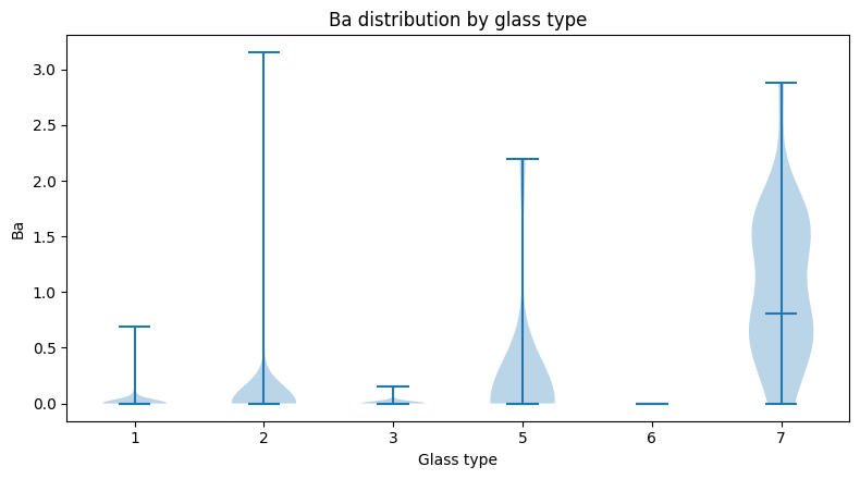
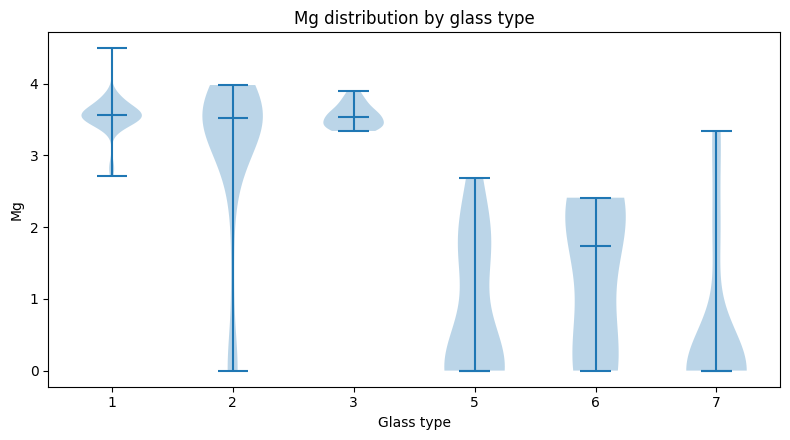
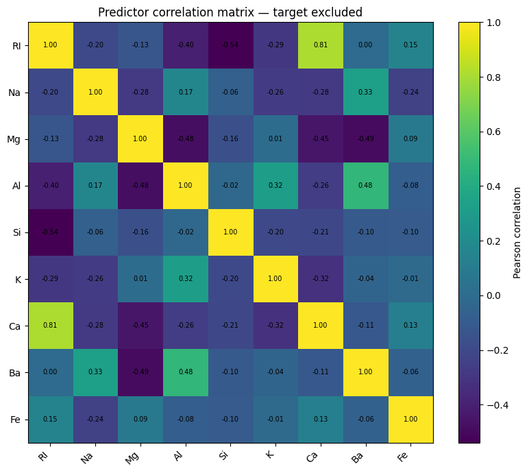
The small size makes a single train/test split too fragile: the 9 tableware samples could almost all land on the same side. The imbalance calls for a metric that gives weight to small classes. And the chemical profiles suggest headlamps and containers will be easier than telling windows apart.
The first method choice follows directly from the small number of samples: how to evaluate.
04 / Evaluating with cross-validation
Five cross-validation folds instead of a single fortunate split.
This frame imposes a strict rule on every preparation step: it must happen inside each fold.
05 / Preparing the data inside each fold
Scale and rebalance, without ever touching the evaluated samples.
If scaling or SMOTE also used the evaluated group, information from that group would leak into training and the score would look artificially good. Evaluated samples therefore always remain real, unseen samples.
With this protocol fixed, I could compare three model families under identical conditions.
06 / Three models compared
A simple model, a neural network and a forest of trees.
Draws linear boundaries between types from the scaled measurements. If it is enough, there is no need to go further.
Two hidden layers with dropout (neurons randomly switched off during training to avoid memorising).
Many decision trees, each learned on a different draw of the data, voting together. Handles non-linear relationships without scaling.
The three models were then evaluated on the same five folds.
07 / Results
Across 213 samples, Random Forest achieves the highest average scores among the models compared.
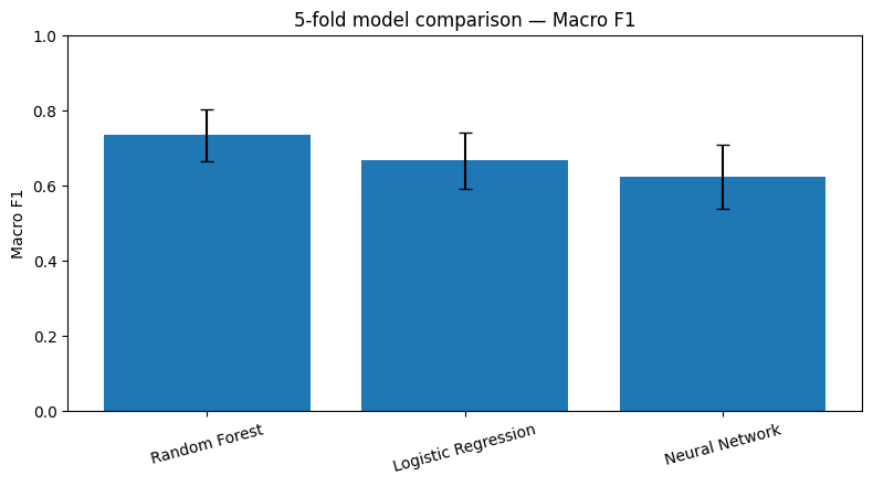
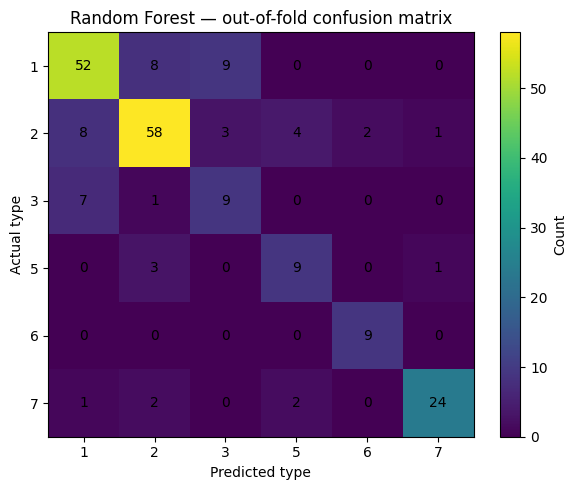
These results say as much about the data as about the models.
08 / Interpretation & real-world value
Match model complexity to the size and shape of the data.
With only 213 samples, the neural network did not perform better under this protocol, while Random Forest can use thresholds between variables, such as magnesium and barium content. Logistic Regression reached 73.0% balanced accuracy but 62.5% overall accuracy: class-balanced evaluation tells a more nuanced story than overall accuracy alone.
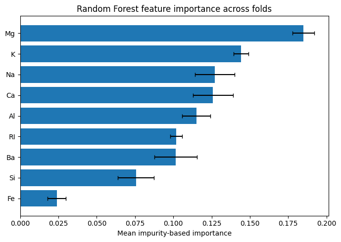
This ranking describes what this model uses to decide; it is not a chemical conclusion about what makes glasses differ.
The model can point an expert to the most likely types for a fragment; it replaces neither laboratory analysis nor forensic interpretation.
Types 1, 2 and 3 have close compositions: that is where more samples or additional measurements would be needed.
These conclusions remain bounded by the size of the dataset.
09 / Limits & lessons
Cross-validation stabilises the evaluation, but it cannot create new data.
- Only 213 samples, 9 of them tableware.
- SMOTE helps learning but does not replace real samples.
- No external dataset to confirm the results.
- Scope: experimental classification using glass chemistry data. The model can guide preliminary analysis; forensic use would require independent validation.
On a small tabular dataset, the evaluation method matters as much as the model. Stratified cross-validation and preparation confined to the folds give modest but credible scores, and they show that a more complex model is not necessarily better.
Going further
I would extend the study with an independent glass dataset, measurements that separate windows better and probability calibration for decision support. The notebook details every step and its outputs.